Power Spectrum Computation

Introduction

The main entry point to the power spectrum module is the calc_power() function, which takes a set of points, deposits them onto a mesh (optionally with interlacing), computes the mode powers through an FFT, and then computes bandpowers and multipoles. This notebook is a quick demonstration of that function, with a similarly quick sanity check against nbodykit.

Example

import numpy as np
import matplotlib.pyplot as plt

from abacusnbody.analysis.power_spectrum import calc_power

Load the data:

power_test_data = dict(**np.load("../../../tests/data_power/test_pos.npz"))
Lbox = 1000.
pos = power_test_data['pos']

Specifications of the power spectrum computation. The only required args are pos and Lbox.

interlaced = True
compensated = True
paste = 'TSC'
nmesh = 72
nbins_mu = 4
logk = False
k_hMpc_max = np.pi*nmesh/Lbox + 1.e-6
nbins_k = nmesh//2
poles = [0, 2, 4]

Compute the power spectrum, including bandpowers and multipoles:

power = calc_power(pos, Lbox, nbins_k, nbins_mu, k_hMpc_max, logk, \
                    paste, nmesh, compensated, interlaced, poles=poles)

The result is an Astropy Table. The shape of the k_avg, power, etc, columns is (nbins_k,nbins_mu). The poles column is shape (nbins_k,len(poles)).

power

Table length=36

k_min	k_max	k_mid	k_avg	power	N_mode	poles	N_mode_poles	mu_min	mu_max	mu_mid
float64	float64	float64	float32[4]	float32[4]	int64[4]	float32[3]	int64	float64[4]	float64[4]	float64[4]
0.0	0.006283213084957364	0.003141606542478682	0.005026548 .. 0.0062831854	7568.9023 .. 6049.0254	5 .. 2	7134.6523 .. 33801.098	7	0.0 .. 0.75	0.25 .. 1.0	0.125 .. 0.875
0.006283213084957364	0.012566426169914728	0.009424819627436047	0.010726068 .. 0.012566371	2942.2803 .. 49420.074	8 .. 2	12721.525 .. 8581.41	26	0.0 .. 0.75	0.25 .. 1.0	0.125 .. 0.875
0.012566426169914728	0.018849639254872094	0.015708032712393412	0.016180087 .. 0.01517894	9128.091 .. 26119.805	16 .. 18	17876.928 .. -4302.0957	90	0.0 .. 0.75	0.25 .. 1.0	0.125 .. 0.875
0.018849639254872094	0.025132852339829457	0.021991245797350775	0.022035956 .. 0.022221854	9138.691 .. 20882.14	20 .. 42	16421.23 .. -2728.3147	134	0.0 .. 0.75	0.25 .. 1.0	0.125 .. 0.875
0.025132852339829457	0.031416065424786824	0.02827445888230814	0.0278653 .. 0.02873107	9497.041 .. 21889.508	80 .. 58	14460.294 .. 1471.5734	258	0.0 .. 0.75	0.25 .. 1.0	0.125 .. 0.875
0.031416065424786824	0.03769927850974419	0.0345576719672655	0.03427213 .. 0.0344824	8653.626 .. 17725.803	112 .. 90	13018.891 .. -5607.4976	410	0.0 .. 0.75	0.25 .. 1.0	0.125 .. 0.875
0.03769927850974419	0.04398249159470155	0.04084088505222287	0.04038116 .. 0.04089897	8631.141 .. 15932.965	108 .. 138	11582.084 .. 430.21402	494	0.0 .. 0.75	0.25 .. 1.0	0.125 .. 0.875
0.04398249159470155	0.050265704679658914	0.04712409813718023	0.046560723 .. 0.04736551	8191.2383 .. 14180.858	144 .. 178	10757.994 .. -2565.6487	690	0.0 .. 0.75	0.25 .. 1.0	0.125 .. 0.875
0.050265704679658914	0.05654891776461628	0.0534073112221376	0.053127706 .. 0.053584747	8125.8447 .. 13207.899	280 .. 226	9751.573 .. -19.154434	962	0.0 .. 0.75	0.25 .. 1.0	0.125 .. 0.875
0.05654891776461628	0.06283213084957365	0.05969052430709496	0.05940248 .. 0.05961299	7919.7124 .. 12426.76	280 .. 274	9381.509 .. 696.6776	1098	0.0 .. 0.75	0.25 .. 1.0	0.125 .. 0.875
...	...	...	...	...	...	...	...	...	...	...
0.16336354020889146	0.16964675329384885	0.16650514675137015	0.16650459 .. 0.16650878	3508.4248 .. 4512.569	2208 .. 2234	3929.0388 .. -230.04236	8994	0.0 .. 0.75	0.25 .. 1.0	0.125 .. 0.875
0.16964675329384885	0.1759299663788062	0.1727883598363275	0.17277633 .. 0.17290868	3562.9634 .. 4224.724	2212 .. 2418	3855.428 .. 27.31195	9446	0.0 .. 0.75	0.25 .. 1.0	0.125 .. 0.875
0.1759299663788062	0.18221317946376356	0.1790715729212849	0.17895347 .. 0.17909919	3525.7412 .. 4377.7456	2600 .. 2458	3806.5596 .. 139.75587	9978	0.0 .. 0.75	0.25 .. 1.0	0.125 .. 0.875
0.18221317946376356	0.18849639254872091	0.18535478600624222	0.185251 .. 0.1852861	3623.513 .. 4494.107	2864 .. 2762	3875.3442 .. 257.82697	11138	0.0 .. 0.75	0.25 .. 1.0	0.125 .. 0.875
0.18849639254872091	0.1947796056336783	0.1916379990911996	0.19156447 .. 0.19152866	3384.806 .. 4229.843	2836 .. 2890	3696.4075 .. 195.4255	11406	0.0 .. 0.75	0.25 .. 1.0	0.125 .. 0.875
0.1947796056336783	0.20106281871863566	0.197921212176157	0.19781813 .. 0.19785866	3382.7285 .. 4218.5186	2960 .. 3186	3763.8347 .. -332.63657	12578	0.0 .. 0.75	0.25 .. 1.0	0.125 .. 0.875
0.20106281871863566	0.207346031803593	0.20420442526111432	0.20413305 .. 0.20423785	3378.4102 .. 4038.1118	3584 .. 3346	3576.4487 .. 61.47841	13490	0.0 .. 0.75	0.25 .. 1.0	0.125 .. 0.875
0.207346031803593	0.2136292448885504	0.2104876383460717	0.21046124 .. 0.21046674	3222.9612 .. 3837.159	3504 .. 3466	3501.6152 .. -58.982677	13962	0.0 .. 0.75	0.25 .. 1.0	0.125 .. 0.875
0.2136292448885504	0.21991245797350775	0.2167708514310291	0.21672955 .. 0.21671747	3282.833 .. 3728.5186	3748 .. 3770	3434.2856 .. 90.5686	15062	0.0 .. 0.75	0.25 .. 1.0	0.125 .. 0.875
0.21991245797350775	0.2261956710584651	0.22305406451598642	0.22298157 .. 0.22308056	3189.86 .. 3806.1758	3702 .. 4002	3485.2192 .. 1.8451325	15688	0.0 .. 0.75	0.25 .. 1.0	0.125 .. 0.875

The meta field saves some information about how the power spectrum was calculated:

power.meta

{'Lbox': 1000.0,
 'logk': False,
 'paste': 'TSC',
 'nmesh': 72,
 'compensated': True,
 'interlaced': True,
 'poles': [0, 2, 4],
 'nthread': 24,
 'N_pos': 421791,
 'is_weighted': False,
 'field_dtype': numpy.float32,
 'squeeze_mu_axis': True}

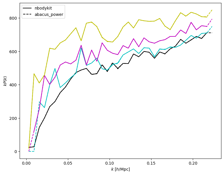
Compare with nbodykit

Load presaved nbodykit computation:

comp_str = "_compensated" if compensated else ""
int_str = "_interlaced" if interlaced else ""
fn = f"../../../tests/data_power/nbody_{paste}{comp_str}{int_str}.npz"
data = np.load(fn)
k_nbody = data['k']
Pkmu_nbody = data['power'].real
Pell_nbody = data['power_ell'].real

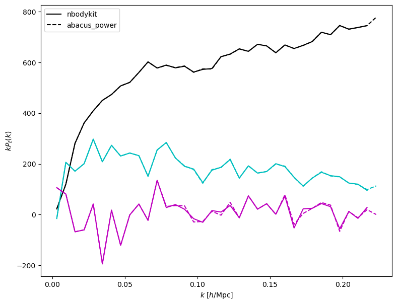
Plot and compare:

colors = ['k', 'c', 'm', 'y']
plt.figure(figsize=(9, 7))
for i in range(nbins_mu):
    if i == 0:
        label1 = 'nbodykit'
        label2 = 'abacus_power'
    else:
        label1 = label2 = None
    plt.plot(k_nbody, Pkmu_nbody[:, i] * k_nbody, c=colors[i], label=label1)
    plt.plot(power['k_mid'], power['power'][:, i] * power['k_mid'], c=colors[i], ls='--', label=label2)
plt.ylabel(r"$k P(k)$")
plt.xlabel(r"$k \ [h/{\rm Mpc}]$")
plt.legend();

# plot and compare
plt.figure(figsize=(9, 7))
for i in range(len(poles)):
    if i == 0:
        label1 = 'nbodykit'
        label2 = 'abacus_power'
    else:
        label1 = label2 = None
    plt.plot(k_nbody, Pell_nbody[i, :] * k_nbody, c=colors[i], label=label1)
    plt.plot(power['k_mid'], power['poles'][:,i] * power['k_mid'], c=colors[i], ls='--', label=label2)
plt.ylabel(r"$k P_\ell(k)$")
plt.xlabel(r"$k \ [h/{\rm Mpc}]$")
plt.legend();