Particle Light Cones

At every timestep, Abacus identifies particles that belong to the light cone and outputs their positions, velocities, particle IDs, and HEALPix pixel number, which can be used to form projected density maps. The pixel orientation is such that the +𝑧 direction coincides with the North Pole. The HEALPix maps are output from all particles with resolution of 𝑁side = 16384, which is more than sufficient for performing accurate weak lensing analysis, whereas the particle outputs contain only a 10% subsample of the particles, the so-called A and B subsamples.

import numpy as np

%matplotlib inline

from mpl_toolkits.mplot3d import Axes3D
import matplotlib.pyplot as plt
import healpy as hp

from abacusnbody.data.read_abacus import read_asdf
from util import histogram_hp

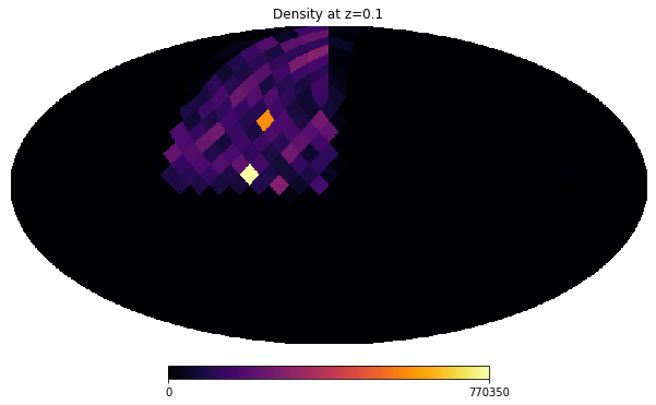
Let’s visualize the HEALPix light cone outputs (containing number of particles per pixel) at the last available global time step (Step 1093), corresponding to z = 0.1.

# simulation directory of light cone outputs
sim_name = 'AbacusSummit_base_c000_ph006'
# NERSC location
f = read_asdf(
    f'/global/project/projectdirs/desi/cosmosim/Abacus//{sim_name:s}/lightcones/heal/LightCone0_heal_Step1093.asdf'
)
print('Redshift = ', f['header']['Redshift'])
print(
    'Observer location relative to all three boxes = ',
    np.array(f['header']['LightConeOrigins']).reshape(-1, 3),
)
heal = f['data']['heal'][:]

Redshift =  0.100969282127725
Observer location relative to all three boxes =  [[ -990.  -990.  -990.]
 [ -990.  -990. -2990.]
 [ -990. -2990.  -990.]]

# plot with healpy in Mollweide projection
nside = 16384  # resolution of healpix maps
npix = hp.nside2npix(nside)
rho = np.zeros(npix, dtype=np.float32)
rho = histogram_hp(rho, heal)

rho = hp.ud_grade(rho, nside_out=8, order_in='NESTED', power=-2)
hp.mollview(rho, nest=True, title='Density at z=0.1', cmap='inferno')

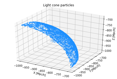
Let’s visualize the positions of the subsampled A and B particles for the original box observer at Step 1093.

# simulation directory of light cone outputs
sim_name = 'AbacusSummit_base_c000_ph006'
# NERSC location
f = read_asdf(
    f'/global/project/projectdirs/desi/cosmosim/Abacus//{sim_name:s}/lightcones/rv/LightCone0_rv_Step1093.asdf'
)
print(f['pos'][:2])
print(f['vel'][:2])

      pos [3]       
--------------------
-920.322 .. -703.782
-920.894 .. -703.562
        vel [3]        
-----------------------
64.453125 .. -32.226562
 73.24219 .. -38.085938

# creating figure
fig = plt.figure()
ax = Axes3D(fig)

# creating the plot
ax.scatter(
    f['pos'][::100, 0], f['pos'][::100, 1], f['pos'][::100, 2], s=1, color='dodgerblue'
)

# setting title and labels
ax.set_title('Light cone particles')
ax.set_xlabel('X [Mpc/h]')
ax.set_ylabel('Y [Mpc/h]')
ax.set_zlabel('Z [Mpc/h]')

Text(0.5, 0, 'Z [Mpc/h]')