Zel’dovich Control Variates (ZCV)#
The purpose of applying the method of Zel’dovich Control Variates (ZCV) to the power spectrum or correlation function multipoles is to reduce the variance on these measurements. Details about the method can be found in Kokron et al. 2022 (arXiv:2205.15327), DeRose et al. 2023 (arXiv:2210.14239) and Hadzhiyska et al. 2023 (in prep.).
Currently, Zel’dovich analytic prediction is only available for the Legendre multipoles ell = 0, 2, 4, so we request that the user specify a subset of those or the full set under poles in power_params. This also implies that nbins_mu in power_params must be set to 1.
Other important ZCV parameters (zcv_params) are nmesh which needs to match nmesh in power_params (the latter can be left blank and will be automatically set in abacus_hod.py). nmesh should also match the number of cells of the initial conditions displacement and density fields (currently, we save nmesh = 576, 1152 for each box). kcut is the Gaussian cut-off scale, which we typically set to half the Nyquist frequency. Finally, fields specifies the Zel’dovich templates that will be used to fit the tracer power spectrum. The full set contains "1cb", "delta", "delta2", "tidal2", "nabla2", and if requesting only a subset of those, the ordering should be contiguous starting with "1cb". Since the Zel’dovich approximation breaks down rather quickly, for most cases, it is sufficient to only include the fields up to "delta" or "delta2". The optional parameter kmax_fit determines the maximum k-value to which we fit the biases. There are also several parameter controlling the smoothness of the CV variable beta (sg_window, dk_window, k0_window and beta1_k), which if not specified, are automatically set to values reasonable for most applications. Note that the function apply_zcv returns the full bias vector, corresponding to b1, b2, bs, bn, shotnoise, where we output zeros for all biases corresponding to fields that are not requested.
When applying ZCV reduction on the correlation function, the following conditions must be met: k_hMpc_max == np.pi*nmesh/Lbox, logk == False, nbins_k == nmesh//2 and n_mu_bins == 1. If not specified by the user, the code should automatically assign these values or output an error message.
The first step in applying the ZCV method is running the “preparation steps.” Below, we provide full instructions for how to do this.
Save the window function (given k-binning) and the Zel’dovich theoretical prediction (given k-binning and redshift):
python -m abacusnbody.hod.zcv.zenbu_window --path2config $1 --alt_simname $2
- If in addition applying ZCV to the correlation function multipoles, run:

`python -m abacusnbody.hod.zcv.zenbu_window --path2config $1 --alt_simname $2 --want_xi`
Save the initial conditions fields (delta, delta^2, s^2, nabla^2):
python -m abacusnbody.hod.zcv.ic_fields --path2config $1 --alt_simname $2
Save the advected fields and their power spectra at this redshift
When applying ZCV to the power spectrum multipoles:
Run this version if planning to use mocks with and without RSD effects:
python -m abacusnbody.hod.zcv.advect_fields --path2config $1 --want_rsd --alt_simname $2Run this version if not planning to use mocks with RSD effects:
python -m abacusnbody.hod.zcv.advect_fields --path2config $1 --alt_simname $2When applying ZCV to the correlation function multipoles:
Run this version if planning to use mocks with and without RSD effects:
python -m abacusnbody.hod.zcv.advect_fields --path2config $1 --want_rsd --alt_simname $2 --save_3D_powerRun this version if not planning to use mocks with RSD effects:
python -m abacusnbody.hod.zcv.advect_fields --path2config $1 --alt_simname $2 --save_3D_power
An example yaml configuration file can be found in the config/ directory, lrg_hod_base_z0.500_nmesh576.yaml. Note that the --alt_simname argument is optional and only needed if the user wants to use a different simulation from the one specified in the yaml file.
# Load necessary packages

import numpy as np
import matplotlib.pyplot as plt
import yaml

from abacusnbody.hod.abacus_hod import AbacusHOD
# Whether to use the last computed tracer power spectra (saves time)
load_presaved = False
# Load the config file and parse in relevant parameters
path2config = 'config/lrg_hod_base_z0.500_nmesh576.yaml'

# Read the parameters from the yaml file
config = yaml.safe_load(open(path2config))
sim_params = config['sim_params']
HOD_params = config['HOD_params']
clustering_params = config['clustering_params']
zcv_params = config['zcv_params']

# Additional parameter choices
want_rsd = HOD_params['want_rsd']
write_to_disk = HOD_params['write_to_disk']
z_mock = sim_params['z_mock']
sim_name = sim_params['sim_name']
nmesh = zcv_params['nmesh']
# Run hod
newBall = AbacusHOD(sim_params, HOD_params, clustering_params)
mock_dict = newBall.run_hod(
    newBall.tracers, want_rsd, write_to_disk=write_to_disk, Nthread=16
)
nobj = mock_dict['LRG']['mass'].size
print('number of galaxies', nobj)
Loading simulation by slab,  0
Loading simulation by slab,  1
Loading simulation by slab,  2
Loading simulation by slab,  3
Loading simulation by slab,  4
Loading simulation by slab,  5
Loading simulation by slab,  6
Loading simulation by slab,  7
Loading simulation by slab,  8
Loading simulation by slab,  9
Loading simulation by slab,  10
Loading simulation by slab,  11
Loading simulation by slab,  12
Loading simulation by slab,  13
Loading simulation by slab,  14
Loading simulation by slab,  15
Loading simulation by slab,  16
Loading simulation by slab,  17
Loading simulation by slab,  18
Loading simulation by slab,  19
Loading simulation by slab,  20
Loading simulation by slab,  21
Loading simulation by slab,  22
Loading simulation by slab,  23
Loading simulation by slab,  24
Loading simulation by slab,  25
Loading simulation by slab,  26
Loading simulation by slab,  27
Loading simulation by slab,  28
Loading simulation by slab,  29
Loading simulation by slab,  30
Loading simulation by slab,  31
Loading simulation by slab,  32
Loading simulation by slab,  33
gen mocks 20.67349934577942
number of galaxies 2851468
# Run zcv on the power spectrum multipoles
zcv_dict = newBall.apply_zcv(mock_dict, config, load_presaved=load_presaved)
print(zcv_dict.keys())
for key in zcv_dict.keys():
    if 'Pk' in key:
        print(key, zcv_dict[key][:, :10])
        print('-----------------')
D =  58.898568747251055
min/max tracer pos 0.0 1999.9994 (2851468, 3)
/global/u1/b/boryanah/repos/abacusutils/abacusnbody/analysis/power_spectrum.py:588: UserWarning: npartition 288 not large enough to use all 256 threads; should be 2*nthread
  tsc_parallel(pos, field, Lbox, weights=w)
field, pos float32 float32
/global/u1/b/boryanah/repos/abacusutils/abacusnbody/analysis/power_spectrum.py:586: UserWarning: npartition 288 not large enough to use all 256 threads; should be 2*nthread
  tsc_parallel(pos + np.float32(d), field, Lbox, weights=w)
shift float32 float32
field fft complex64
Computing auto-correlation of tracer
Computing cross-correlation of tracer and  1cb
Computing cross-correlation of tracer and  delta
gen mocks 0.46642112731933594
D =  58.898568747251055
min/max tracer pos 0.00012207031 1999.9994 (2851468, 3)
/global/u1/b/boryanah/repos/abacusutils/abacusnbody/analysis/power_spectrum.py:588: UserWarning: npartition 288 not large enough to use all 256 threads; should be 2*nthread
  tsc_parallel(pos, field, Lbox, weights=w)
field, pos float32 float32
/global/u1/b/boryanah/repos/abacusutils/abacusnbody/analysis/power_spectrum.py:586: UserWarning: npartition 288 not large enough to use all 256 threads; should be 2*nthread
  tsc_parallel(pos + np.float32(d), field, Lbox, weights=w)
shift float32 float32
field fft complex64
Computing auto-correlation of tracer
Computing cross-correlation of tracer and  1cb
Computing cross-correlation of tracer and  delta
zeros in the measured power spectra =  0 3456 864
zeros in the measured power spectra =  0 10368 2592
bias [1.00000000e+00 9.91593878e-01 0.00000000e+00 0.00000000e+00
 0.00000000e+00 4.40394709e+03]
dict_keys(['k_binc', 'poles', 'rho_tr_ZD', 'rho_tr_ZD_sn_lim', 'Pk_ZD_ZD_ell', 'Pk_tr_ZD_ell', 'Pk_tr_tr_ell', 'Nk_tr_tr_ell', 'Pk_tr_tr_ell_zcv', 'Pk_ZD_ZD_ell_ZeNBu', 'bias'])
Pk_ZD_ZD_ell [[ 51846.4118589   28547.01288313  63369.3990674   65156.66968237
   73664.75750497  68726.76759015  66153.33595083  71303.95179111
   58044.78112957  53687.82978115]
 [217186.81095903  16981.44693907  30356.36199179  78428.67031589
   29731.83492904  33525.4805439   31147.88947603  40479.78992266
   16639.779122    18464.40769471]
 [435083.80210592  -7306.50971393 -25077.74117642   -598.28280476
   23294.92010325 -18654.5527025    4657.03811136   -757.03161118
  -18626.10989175  -6809.6146928 ]]
-----------------
Pk_tr_ZD_ell [[ 5.32928956e+04  2.90608301e+04  6.54554818e+04  6.66062788e+04
   7.45350005e+04  7.09860277e+04  6.83537785e+04  7.35341995e+04
   6.03593707e+04  5.54929005e+04]
 [ 2.23350629e+05  1.57414281e+04  3.23016957e+04  8.09235651e+04
   3.12185001e+04  3.44826745e+04  3.28481396e+04  4.25054341e+04
   1.49095882e+04  1.97380728e+04]
 [ 4.47300685e+05 -8.13513155e+03 -2.56254995e+04 -3.70018946e+01
   2.49900939e+04 -1.93424269e+04  7.27587802e+03  2.04772601e+03
  -2.03131178e+04 -6.09422956e+03]]
-----------------
Pk_tr_tr_ell [[ 55948.73046875  31177.73242188  68993.4609375   69842.3515625
   77214.65625     75257.640625    72410.8125      77926.7890625
   64913.05078125  59304.62109375]
 [231579.796875    13986.83300781  34373.32421875  82460.2578125
   32536.8203125   35820.16015625  34958.921875    44444.4765625
   13316.60839844  21234.91796875]
 [467415.6875      -8596.67089844 -27467.90039062    480.84347534
   27301.78125    -20495.49023438  10121.4609375    4853.46875
  -22127.70507812  -5206.25976562]]
-----------------
Pk_tr_tr_ell_zcv [[ 2920.1479991  43237.91252416 61742.15462507 69873.73176211
  72749.24444374 76187.90388097 74525.45975927 71166.74496517
  66616.77981931 61661.2517163 ]
 [14276.91845587 13247.57225672 28310.05440666 33619.10086385
  34055.28660063 32737.53494706 35840.09791595 32346.78562168
  22755.90359715 27929.49404126]
 [30681.13341979 -2494.4419015  -2887.68305845   961.75140763
   6366.45699668 -2534.18337934  8882.41878456  5970.34419963
  -2443.41031284  3026.25371553]]
-----------------
Pk_ZD_ZD_ell_ZeNBu [[-1069.0522981  40585.41234184 56125.00353158 65188.05714889
  69192.41159538 69659.6485993  68276.05331773 64514.4358319
  59755.74139132 56052.17275136]
 [  534.52614905 16243.66920644 24297.33594445 29550.57600351
  31253.63047216 30432.26063124 32032.86869649 28325.77427263
  26119.50486962 25179.25652399]
 [ -400.89436109 -1216.31249936  -515.55894428  -117.04771289
   2315.69565446  -633.23901606  3412.74836313   364.98394498
   1142.14102421  1448.00903846]]
-----------------
# Run zcv on the correlation function multipoles
zcv_dict_xi = newBall.apply_zcv_xi(mock_dict, config, load_presaved=load_presaved)
print(zcv_dict_xi.keys())
for key in zcv_dict_xi.keys():
    if 'Xi' in key:
        print(key, zcv_dict_xi[key][:, :10])
        print('-----------------')
D =  58.898568747251055
min/max tracer pos 0.0 1999.9994 (2851468, 3)
field, pos float32 float32
shift float32 float32
field fft complex64
Computing auto-correlation of tracer
Computing cross-correlation of tracer and  1cb
Computing cross-correlation of tracer and  delta
gen mocks 0.46341633796691895
D =  58.898568747251055
min/max tracer pos 0.00012207031 1999.9994 (2851468, 3)
field, pos float32 float32
shift float32 float32
field fft complex64
Computing auto-correlation of tracer
Computing cross-correlation of tracer and  1cb
Computing cross-correlation of tracer and  delta
/global/u1/b/boryanah/repos/abacusutils/abacusnbody/hod/zcv/tools_cv.py:592: UserWarning: Setting the parameters correctly for Xi computation
  warnings.warn("Setting the parameters correctly for Xi computation")
Projecting 1cb 1cb
Projecting delta 1cb
Projecting delta delta
bias [1.00000000e+00 9.97573409e-01 0.00000000e+00 0.00000000e+00
 0.00000000e+00 5.30406033e-07]
Compressed
dict_keys(['k_binc', 'poles', 'rho_tr_ZD', 'Pk_ZD_ZD_ell', 'Pk_tr_ZD_ell', 'Pk_tr_tr_ell', 'Nk_tr_tr_ell', 'Pk_tr_tr_ell_zcv', 'Pk_ZD_ZD_ell_ZeNBu', 'bias', 'Xi_tr_tr_ell_zcv', 'Xi_tr_tr_ell', 'Np_tr_tr_ell', 'r_binc'])
Xi_tr_tr_ell_zcv [[  81.43629       0.            0.            5.4717236     3.7121673
     0.            2.689001      1.178847      1.2678285     1.2842284 ]
 [-203.59071       0.            0.            4.2962055    -0.35421377
     0.            0.8991501    -0.54169625   -0.27910763   -0.31785497]
 [ 274.84747       0.            0.           31.948708     -4.2080684
     0.            3.1925206     1.3314441    -1.6291361    -1.0895718 ]]
-----------------
Xi_tr_tr_ell [[  81.40318       0.            0.            5.5085707     3.7155805
     0.            2.6903267     1.1835886     1.274286      1.2897264 ]
 [-203.50797       0.            0.            4.307762     -0.35481212
     0.            0.9038338    -0.53515244   -0.27759308   -0.3145048 ]
 [ 274.73575       0.            0.           32.150814     -4.211427
     0.            3.190259      1.3349391    -1.637801     -1.1030693 ]]
-----------------
# Parse the output from the ZCV-reduced power spectrum measurements
k_binc = zcv_dict['k_binc']
pk_nn_betasmooth = zcv_dict['Pk_tr_tr_ell_zcv']
pk_tt_poles = zcv_dict['Pk_tr_tr_ell']
pk_zz = zcv_dict['Pk_ZD_ZD_ell']
pk_zn = zcv_dict['Pk_tr_ZD_ell']
r_zt = zcv_dict['rho_tr_ZD']
pk_zenbu = zcv_dict['Pk_ZD_ZD_ell_ZeNBu']
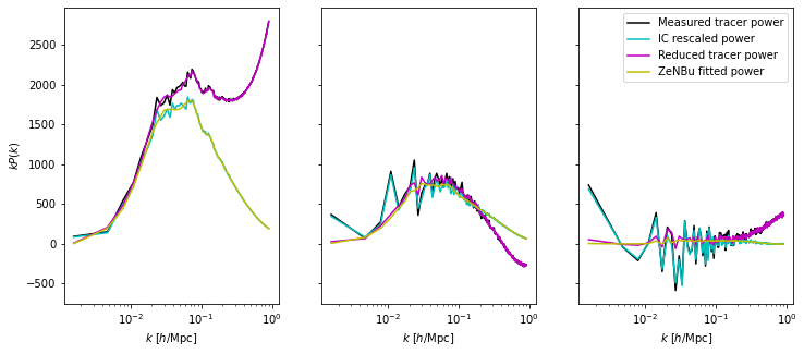
Plot the ZCV reduction on the power spectrum.
# Set up the canvas
cs = ['k', 'c', 'm', 'y']
if want_rsd:
    figsize = (12, 5)
    n_ell = 3
else:
    figsize = (6, 5)
    n_ell = 1
f, ax = plt.subplots(1, n_ell, sharex=True, sharey=True, figsize=figsize)
if not want_rsd:
    ax = [ax]

# Loop over all multipoles
for ell in range(n_ell):
    if want_rsd:
        pk_zz_ell = pk_zz[ell, :].flatten()
        pk_zenbu_ell = pk_zenbu[ell, :].flatten()
        pk_tt_poles_ell = pk_tt_poles[ell, :]
        pk_nn_betasmooth_ell = pk_nn_betasmooth[ell, :]
    else:
        pk_zz_ell = pk_zz.flatten()
        pk_zenbu_ell = pk_zenbu.flatten()
        pk_tt_poles_ell = pk_tt_poles.flatten()
        pk_nn_betasmooth_ell = pk_nn_betasmooth.flatten()

    ax[ell].plot(
        k_binc, k_binc * pk_tt_poles_ell, c=cs[0], label='Measured tracer power'
    )
    ax[ell].plot(k_binc, k_binc * pk_zz_ell, c=cs[1], label='IC rescaled power')
    ax[ell].plot(
        k_binc, k_binc * pk_nn_betasmooth_ell, c=cs[2], label='Reduced tracer power'
    )
    ax[ell].plot(k_binc, k_binc * pk_zenbu_ell, c=cs[3], label='ZeNBu fitted power')

    if ell == 0:
        ax[ell].set_ylabel(r'$k P(k)$')
    ax[ell].set_xlabel(r'$k \ [h/{\rm Mpc}]$')
plt.xscale('log')
plt.legend()
<matplotlib.legend.Legend at 0x7f10b3156a10>
# read ZCV output
r_binc = zcv_dict_xi['r_binc']
xi = zcv_dict_xi['Xi_tr_tr_ell_zcv'].reshape(3, len(r_binc))
xi_raw = zcv_dict_xi['Xi_tr_tr_ell'].reshape(3, len(r_binc))

# plot Xi
n_ell = 3
figsize = (14, 6)
f, ax = plt.subplots(1, n_ell, sharex=True, sharey=True, figsize=figsize)
for ell in range(n_ell):
    ax[ell].plot(r_binc, xi[ell] * r_binc**2, cs[1], label='IFT[P(k)] CV')
    ax[ell].plot(r_binc, xi_raw[ell] * r_binc**2, cs[2], label='IFT[P(k)] Raw')
    ax[ell].set_xlabel(r'$r \ [{\rm Mpc}/h]$')
    if ell == 0:
        ax[ell].set_ylabel(r'$\xi_\ell(r) \  r^2 \ [{\rm Mpc}/h]$')
plt.legend(fontsize=16)
plt.ylim([-100, 120])
plt.xlim([1, 200])
(1.0, 200.0)
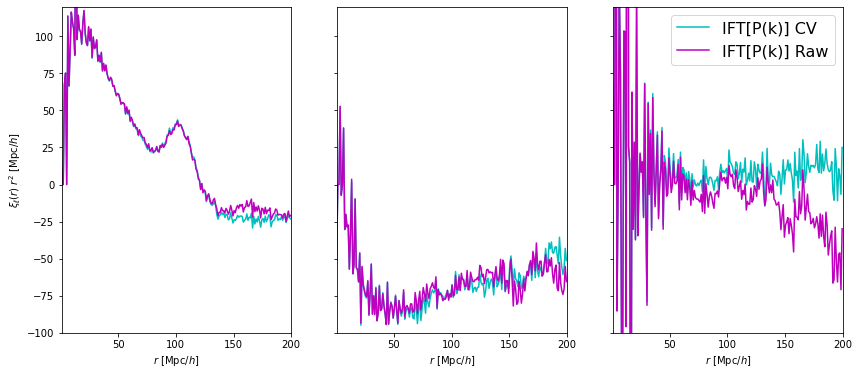
Note that inverse Fourier transforming the 3D power spectrum into a 3D Xi and converting those into Legendre polynomials introduces a lot of noise on small scales. For this reason, we recommend supplementing the correlation function measurement below r <= 50 Mpc/h with a brute-force pair counting using e.g., Corrfunc.
# sqrt(1-rho_xc^2) gives the ratio between the ZCV and the Raw power spectrum uncertainty for each Legendre multipole
print(np.sqrt(1.0 - r_zt[:, :30] ** 2))
[[0.16846982 0.30437687 0.19713057 0.18258624 0.21017712 0.22234371
  0.21804134 0.22258909 0.25436922 0.25164304 0.24893422 0.27187299
  0.27735938 0.29015287 0.30092472 0.29845907 0.31286193 0.32362094
  0.33934459 0.3469444  0.33348162 0.34586629 0.36324817 0.35830913
  0.3679379  0.38109333 0.38604798 0.40631136 0.40804444 0.41671472]
 [0.16630195 0.29242323 0.16487771 0.13634753 0.19396959 0.21415448
  0.20548919 0.19656067 0.26416445 0.24664422 0.24988234 0.25001118
  0.26720739 0.27884409 0.29260717 0.26957729 0.30016282 0.30055123
  0.31954065 0.3296279  0.3176188  0.33296158 0.35374401 0.33843627
  0.35023992 0.36286843 0.37358073 0.38995422 0.39068864 0.40601641]
 [0.16726483 0.29139558 0.17743489 0.1446058  0.19499308 0.21570578
  0.2079886  0.20136724 0.25884142 0.24660162 0.24552127 0.2527322
  0.26801824 0.28104147 0.29267271 0.2733443  0.30187102 0.30445232
  0.32146398 0.33255927 0.31979706 0.33386936 0.35356322 0.34100628
  0.35396408 0.36518434 0.37461326 0.39232893 0.39283278 0.40633439]]