Using Subsample Particles with CompaSO Halos#
Background#
In AbacusSummit, every particle falls into one of three sets:
subsample A (3%)
subsample B (7%)
not a subsample particle
Membership in these sets is determined by a hash of the particle ID, and so is consistent across time (and even between simulations, roughly speaking). Since the set of A and B particles is disjoint, the union of the two sets produces a 10% subsample.
When a CompaSO halo is found, any subsample A or B particles in that halo are appended to an array, which is output as a data product alongside the halo catalog. A and B particles go into separate arrays, and these arrays are saved in separate files (with names like halo_rv_A or halo_pid_B). Each halo catalog entry (record) contains the indexing information needed to find its subsample particles in those arrays. The CompaSOHaloCatalog interface uses that information to load the particles transparently when the user asks for them.
In particular, these outputs were designed with HOD applications in mind. For example, the AbacusHOD module uses these subsample particles to help determine where to place HOD tracers. Many HOD applications will only need the A subsample, so we’ll focus on them in this notebook.
What if I want all particles in a halo?#
While a limited number of simulations have full timeslice outputs (i.e. 100% particle outputs), the data model is such that the assocation between halos and particles in the full timeslices is not saved. New halo finding could be run on the full timeslices, but in general, only the A and B subsamples are available for a halo.
Loading and Plotting the Subsamples#
This notebook walks through loading subsample particles and doing some plotting and sanity checks to help users understand the data model.
We’ll start with the basic imports:
from pathlib import Path

import matplotlib
import matplotlib.pyplot as plt
import numpy as np

from abacusnbody.data.compaso_halo_catalog import CompaSOHaloCatalog
We’ll next load the halo catalog. We’ll use the mini simulation included in the test data, so this notebook can be run without downloading AbacusSummit data. We’ll use the subsamples parameter to indicate we want the A subsample particles.
catdir = Path('../../../tests/Mini_N64_L32/halos/z0.000')
cat = CompaSOHaloCatalog(catdir, subsamples=dict(A=True))
print(cat)
CompaSO Halo Catalog
====================
Mini_N64_L32 @ z=0
------------------
     Halos:      381 halos,      91 fields, 0.000244 GB
Subsamples: 2.54e+03 particles,   2 fields, 6.09e-05 GB
Cleaned halos: True
Halo light cone: False
We see we have a small simulation with 381 halos and ~2540 subsample particles.
Is that about the right number of particles? It should be about 3% of the total particles in halos (the fraction 0.03 is stored in the ParticleSubsampleA parameter):
cat.halos['N'].sum() * cat.header['ParticleSubsampleA']
2549.46
2549 matches well with our expectation.
Now let’s look at the subsamples themselves:
cat.subsamples
| pos | vel |
|---|---|
| float32[3] | float32[3] |
| -14.187456 .. -5.318592 | 477.53906 .. 108.39844 |
| -14.207712 .. -5.357984 | 228.51562 .. -190.42969 |
| -14.151616 .. -5.303104 | 421.875 .. -117.1875 |
| -14.161888 .. -5.317536 | 342.77344 .. -149.41406 |
| -14.237088 .. -5.25504 | 433.59375 .. -225.58594 |
| -14.181344 .. -5.272928 | 483.39844 .. -210.9375 |
| -14.190272 .. -5.247936 | 489.2578 .. -166.99219 |
| -14.398592 .. -4.653216 | 249.02344 .. 187.5 |
| -13.870208 .. -4.550208 | 404.29688 .. 149.41406 |
| -15.16832 .. -4.958496 | 404.29688 .. 260.7422 |
| ... | ... |
| 15.292704 .. -2.744448 | 158.20312 .. 178.71094 |
| 15.220832 .. -2.755104 | 149.41406 .. 117.1875 |
| 15.353792 .. -11.705376 | -41.015625 .. 175.78125 |
| 15.35824 .. -11.625824 | 281.25 .. 389.64844 |
| 15.334656 .. -11.635968 | -38.085938 .. 114.25781 |
| 15.362496 .. -11.654432 | -17.578125 .. 84.96094 |
| 15.421216 .. -11.658336 | -175.78125 .. 93.75 |
| -15.958912 .. -3.628928 | 210.9375 .. -58.59375 |
| 15.914784 .. -3.701504 | 454.10156 .. -67.38281 |
| 15.937216 .. -3.75104 | 231.44531 .. -79.10156 |
We have two columns, pos and vel, each of which is an array of shape (N,3). The units of pos are Mpc/h (where the center of the box is at (0,0,0), so the positions span [-L/2,L/2]), and the units of velocities are proper km/s.
Let’s plot the halo field and the subsample particles and check that they trace out the same large-scale structure. This simulation is pretty low resolution, so the LSS isn’t that strong, but it should be visible.
L = cat.header['BoxSize']
fig, ax = plt.subplots(dpi=150)
ax.set_aspect('equal')
ax.set_xlim(-L / 2, L / 2)
ax.set_ylim(-L / 2, L / 2)

ax.scatter(
    cat.subsamples['pos'][:, 0],
    cat.subsamples['pos'][:, 1],
    s=10.0,
    label='Subsample particles',
)
ax.scatter(
    cat.halos['x_L2com'][:, 0],
    cat.halos['x_L2com'][:, 1],
    s=1.0,
    label='Halo centers',
)
ax.set_xlabel('$x$ [Mpc/$h$]')
ax.set_ylabel('$y$ [Mpc/$h$]')

ax.legend(loc='upper right')
<matplotlib.legend.Legend at 0x7f81b2182d30>
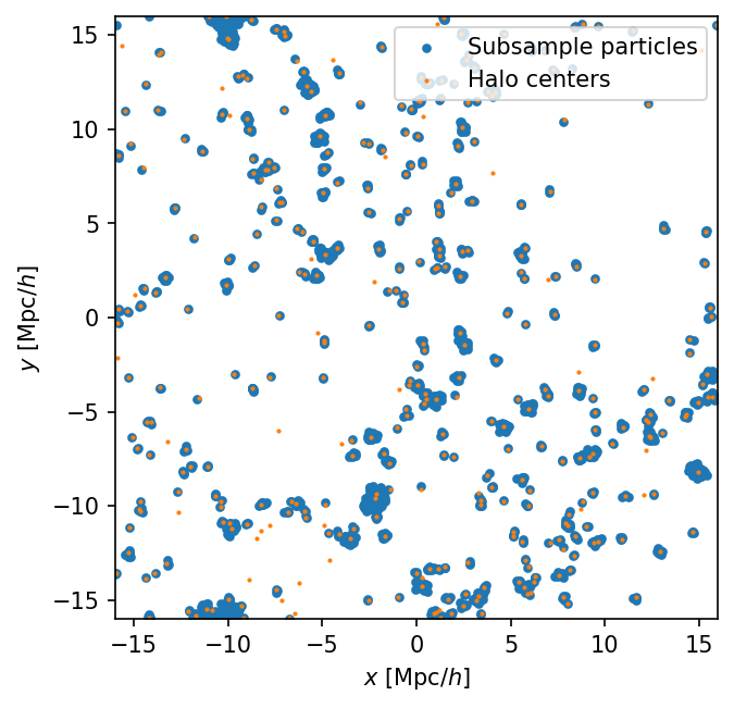
The two are in excellent agreement. We see some halos without subsamples, which is fine, and no subsamples that are missing halos seem to stand out, which is good.
Finding a halo’s subsample particles#
The subsample particles come in one big array, ordered by halo. So all we need to know is the starting index and count of subsample particles that belong to a halo. In the halo catalog, the starting index is called npstartA and the count is called npoutA.
Let’s pick a big halo and use these indices to get its subsample particles:
bighalo = cat.halos[123]
print(bighalo['N'])
print(bighalo['x_L2com'])
287
[-6.0305486 13.056745  -9.907915 ]
bighalo_subsamples = cat.subsamples[
    bighalo['npstartA'] : bighalo['npstartA'] + bighalo['npoutA']
]
bighalo_subsamples['pos'].data  # using .data just so all three columns are printed
array([[-5.99168 , 13.059168, -9.909504],
       [-5.931904, 13.031616, -9.931072],
       [-6.07488 , 13.055808, -9.810816],
       [-6.037824, 13.102976, -9.973056]], dtype=float32)
We see that all 4 subsample particles are within a few 10s of kpc/h of the halo center, as we would expect. Having only 4 subsample particles is a bit unusual for a halo with 287 particles; we might expect 8.6 on average, but it’s a reasonable Poisson fluctuation.
L0 Halo Particles#
One potentially surprising feature of the subsample data model is that there are more subsample particles in the subsample files than the halos think they should have. For technical reasons, this is hidden from the user through the Python interface, but we can see it if we load the files directly:
def count_raw_subsamples():
    import asdf

    count = 0
    for fn in (catdir / 'halo_rv_A').glob('halo_rv_A_*.asdf'):
        with asdf.open(fn) as af:
            count += len(af['data']['rvint'])
    return count


print(count_raw_subsamples())
print(cat.halos['npoutA'].sum())
2975
2536
So there are about 440 extra, unindexed subsample particles. These are L0 particles: particles that were part of the density-bounded FoF groups that form the first level of segmentation in the CompaSO algorithm. Within each L0 group, multiple halos (L1 groups) can be identified, but not all particles may belong to L1 halos. These L0-but-not-L1 particles are the unindexed extras.
Most users will never encounter this, unless one is inspecting the raw ASDF files.
Cleaned Subsample Particles#
The halo “cleaning” procedure assigns the mass of one halo to another. The halo that was “cleaned away” is assigned an N of 0. The subsample particle count is likewise set to 0, and the halo to which it is merged gains those particles in its subsample. This is all transparent to the user.
However, we can still load the uncleaned halo catalogs and see this reassignment of subsample particles in action for pedagogical purposes. In this small sim, we only have 1 halo that was cleaned away:
removed_idx = (cat.halos['N'] == 0).argmax()
removed = cat.halos[removed_idx]
removed['N', 'npoutA']
| N | npoutA |
|---|---|
| uint32 | uint32 |
| 0 | 0 |
It we can use the haloindex to find the halo it was merged to:
mergedto_idx = (cat.halos['haloindex'] == removed['is_merged_to']).argmax()
mergedto = cat.halos[mergedto_idx]
mergedto['N', 'npoutA']
| N | npoutA |
|---|---|
| uint32 | uint32 |
| 205 | 3 |
And we can look back in the uncleaned catalog to see how many of those particles and subsample particles came from the cleaning:
catunclean = CompaSOHaloCatalog(catdir, subsamples=dict(A=True), cleaned=False)
catunclean.halos[removed_idx]['N', 'npoutA']
| N | npoutA |
|---|---|
| uint32 | uint32 |
| 60 | 3 |
catunclean.halos[mergedto_idx]['N', 'npoutA']
| N | npoutA |
|---|---|
| uint32 | uint32 |
| 145 | 0 |
So in this case, all 3 of the subsample particles came from the merged object. A bit unusual, but the original object only had a Poisson expectation of 145*0.03 = 4.35 subsample A particles.
Subsample Particle PIDs#
So far, we have only looked at subsample particle positions, but the PID field (really, the aux field) of the particles encodes a lot of information, too. We can tell abacusutils to load the PIDs with subsamples=dict(pid=True), and then unpack all aux-derived fields with unpack_bits=True:
cat = CompaSOHaloCatalog(
    catdir, subsamples=dict(A=True, rv=True, pid=True), unpack_bits=True
)
cat.subsamples
| pid | lagr_pos | lagr_idx | tagged | density | pos | vel |
|---|---|---|---|---|---|---|
| int64 | float32[3] | int16[3] | bool | float32 | float32[3] | float32[3] |
| 141737852987 | 13.5 .. 0.5 | 59 .. 33 | True | 576.0 | -14.187456 .. -5.318592 | 477.53906 .. 108.39844 |
| 158917918782 | 15.0 .. 2.5 | 62 .. 37 | True | 484.0 | -14.207712 .. -5.357984 | 228.51562 .. -190.42969 |
| 137439019066 | 13.0 .. 0.0 | 58 .. 32 | True | 484.0 | -14.151616 .. -5.303104 | 421.875 .. -117.1875 |
| 137443082298 | 13.0 .. 0.0 | 58 .. 32 | True | 484.0 | -14.161888 .. -5.317536 | 342.77344 .. -149.41406 |
| 150327918652 | 14.0 .. 1.5 | 60 .. 35 | True | 400.0 | -14.237088 .. -5.25504 | 433.59375 .. -225.58594 |
| 141737984060 | 14.0 .. 0.5 | 60 .. 33 | True | 256.0 | -14.181344 .. -5.272928 | 483.39844 .. -210.9375 |
| 146032951356 | 14.0 .. 1.0 | 60 .. 34 | True | 324.0 | -14.190272 .. -5.247936 | 489.2578 .. -166.99219 |
| 68720066623 | 15.5 .. -8.0 | 63 .. 16 | True | 256.0 | -14.398592 .. -4.653216 | 249.02344 .. 187.5 |
| 60129869883 | 13.5 .. -9.0 | 59 .. 14 | True | 484.0 | -13.870208 .. -4.550208 | 404.29688 .. 149.41406 |
| 21475360828 | 14.0 .. -13.5 | 60 .. 5 | False | 225.0 | -15.16832 .. -4.958496 | 404.29688 .. 260.7422 |
| ... | ... | ... | ... | ... | ... | ... |
| 124556607550 | 15.0 .. -1.5 | 62 .. 29 | True | 729.0 | 15.292704 .. -2.744448 | 158.20312 .. 178.71094 |
| 115966607420 | 14.0 .. -2.5 | 60 .. 27 | True | 625.0 | 15.220832 .. -2.755104 | 149.41406 .. 117.1875 |
| 12887785472 | -16.0 .. -14.5 | 0 .. 3 | True | 784.0 | 15.353792 .. -11.705376 | -41.015625 .. 175.78125 |
| 17182818365 | 14.5 .. -14.0 | 61 .. 4 | True | 961.0 | 15.35824 .. -11.625824 | 281.25 .. 389.64844 |
| 4297982011 | 13.5 .. -15.5 | 59 .. 1 | True | 900.0 | 15.334656 .. -11.635968 | -38.085938 .. 114.25781 |
| 4297850941 | 14.5 .. -15.5 | 61 .. 1 | True | 961.0 | 15.362496 .. -11.654432 | -17.578125 .. 84.96094 |
| 12887523391 | 15.5 .. -14.5 | 63 .. 3 | True | 784.0 | 15.421216 .. -11.658336 | -175.78125 .. 93.75 |
| 98787852343 | 11.5 .. -4.5 | 55 .. 23 | False | 121.0 | -15.958912 .. -3.628928 | 210.9375 .. -58.59375 |
| 107377786937 | 12.5 .. -3.5 | 57 .. 25 | True | 400.0 | 15.914784 .. -3.701504 | 454.10156 .. -67.38281 |
| 111672623160 | 12.0 .. -3.0 | 56 .. 26 | True | 324.0 | 15.937216 .. -3.75104 | 231.44531 .. -79.10156 |
We see a few useful fields. lagr_pos is the Lagrangian position of the particle (i.e. the location in the initial particle grid). Therefore the following are the Lagrangian displacements, taking care to wrap any particles that cross the periodic boundary:
lagr_disp = cat.subsamples['pos'] - cat.subsamples['lagr_pos']
lagr_disp[lagr_disp >= L / 2] -= L
lagr_disp[lagr_disp < -L / 2] += L
lagr_disp
| 4.312544 .. -5.818592 |
| 2.7922878 .. -7.857984 |
| 4.848385 .. -5.303104 |
| 4.838112 .. -5.317536 |
| 3.7629128 .. -6.75504 |
| 3.818657 .. -5.772928 |
| 3.8097267 .. -6.247936 |
| 2.101408 .. 3.346784 |
| 4.6297913 .. 4.449792 |
| 2.8316803 .. 8.541504 |
| 2.6740494 .. 8.070976 |
| 2.6552963 .. 8.0655365 |
| ... |
| 1.1534405 .. -1.6241283 |
| -0.5254402 .. -1.6979523 |
| 0.29270363 .. -1.244448 |
| 1.2208319 .. -0.25510406 |
| -0.6462078 .. 2.7946243 |
| 0.8582401 .. 2.374176 |
| 1.8346558 .. 3.8640318 |
| 0.8624964 .. 3.8455677 |
| -0.07878399 .. 2.8416643 |
| 4.541088 .. 0.87107205 |
| 3.4147844 .. -0.20150399 |
| 3.9372158 .. -0.75104 |
The lagr_idx field is the 3D index of the particle in the initial lattice (lagr_pos is computed from this).
The tagged field is used for merger tracking (tagged particles were once part of an L2 halo).
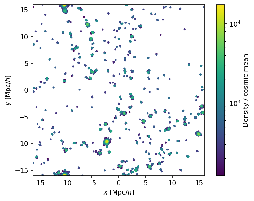
The density field is a KDE estimate in units of the mean density (radius cat.header['DensityKernelRad'] = 0.4, units of initial particle spacing). We expect particles in clustered regions to have a higher density; we can plot them to see this. We’ll make reordered copy of the subsamples to plot the denser particles on top, and apply a log stretch:
fig, ax = plt.subplots(dpi=150)
ax.set_aspect('equal')
ax.set_xlim(-L / 2, L / 2)
ax.set_ylim(-L / 2, L / 2)
ax.set_xlabel('$x$ [Mpc/$h$]')
ax.set_ylabel('$y$ [Mpc/$h$]')
subsamp_densorder = cat.subsamples[cat.subsamples['density'].argsort()]

sc = ax.scatter(
    subsamp_densorder['pos'][:, 0],
    subsamp_densorder['pos'][:, 1],
    s=4.0,
    c=subsamp_densorder['density'],
    norm=matplotlib.colors.LogNorm(),
)
cbar = fig.colorbar(sc)
cbar.set_label('Density / cosmic mean')
Efficiently using the indexing data model#
The Numpy Way#
Here’s a simple question: what is the most distant subsample particle from its halo center? To compute this efficiently in the Numpy world that we’re used to, we would try to solve this problem by broadcasting (or really just by making array shapes match). This is not the most efficient way to solve this problem, but we’ll demonstrate it first.
We have an array of halo centers of shape (Nh,3), and an array of particle positions (Np,3). So we need to repeat each halo position as many times as it has subsample particles:
repeats = np.repeat(cat.halos['x_L2com'], cat.halos['npoutA'], axis=0)
dist = cat.subsamples['pos'] - repeats
dist[dist >= L / 2] -= L
dist[dist <= -L / 2] += L
dist
| -0.008805275 .. -0.00019741058 |
| -0.029061317 .. -0.039589405 |
| 0.02703476 .. 0.015290737 |
| 0.016762733 .. 0.0008587837 |
| -0.058437347 .. 0.06335449 |
| -0.0026931763 .. 0.045466423 |
| -0.011621475 .. 0.07045889 |
| -0.014734268 .. 0.027872562 |
| 0.040781975 .. 0.049615383 |
| 0.1417551 .. 0.078384876 |
| -0.01587677 .. 0.10785675 |
| -0.034628868 .. 0.10241699 |
| ... |
| 0.017808914 .. -0.07621002 |
| -0.16107178 .. -0.15003395 |
| -0.0010995865 .. 0.0043182373 |
| -0.072971344 .. -0.006337881 |
| -0.014093399 .. -0.054498672 |
| -0.009645462 .. 0.025053024 |
| -0.033229828 .. 0.014908791 |
| -0.0053892136 .. -0.0035552979 |
| 0.05333042 .. -0.007458687 |
| 0.13964462 .. 0.0899272 |
| 0.013339996 .. 0.01735115 |
| 0.03577137 .. -0.03218484 |
np.sqrt((dist**2).sum(-1)).max()
0.9396648
So the most distant subsample particle is about 1 Mpc/h away from its halo center, which is very reasonable.
Note that we didn’t actually need to use npstartA in this approach, because the subsample particles appear in catalog order (the 1 halo removed for cleaning has a special npstartA value, but a zero npoutA so it doesn’t matter):
(cat.halos['npoutA'].cumsum()[:-1] != cat.halos['npstartA'][1:]).sum()
1
The Numba Way#
In the Numpy way, we had to construct a large intermediate array (repeats) to do this calculation. For a small example like this, that was okay, but when the subsample particle data is in the 10s of GB, you won’t want to create another array that’s also 10s of GB, when you could have computed it on the fly. The numpy approach forces you to construct an intermediate array, which is both slower and less memory efficient.
An alternative is a procedural approach rather than an array-oriented approach. Numba is a good tool for doing this in Python. Here’s how we would solve the farthest-particle problem in Numba:
import numba


@numba.njit
def find_farthest(halos, particles, counts):
    k = 0
    maxdist = np.float32(-1.0)
    for i in range(len(halos)):
        cen = halos[i]
        for j in range(counts[i]):
            diff = cen - particles[k + j]
            for m in range(len(diff)):
                if diff[m] > L / 2:
                    diff[m] -= L
                if diff[m] < -L / 2:
                    diff[m] += L
            dist = np.sqrt((diff**2).sum(-1))
            if dist > maxdist:
                maxdist = dist
        k += counts[i]
    return maxdist


find_farthest(cat.halos['x_L2com'], cat.subsamples['pos'], cat.halos['npoutA'])
0.9396647810935974
It gives the same result as Numpy, as we expect. It’s a fair bit lengthier, but the code is all pretty simple. So the Numpy approach is fine for small sims, but for applications where memory usage or performance are concerned, an approach like this one that avoids creating intermediate arrays like should be preferred.
numba also lends itself well to parallelization; one could use similar code, parallelizing the outer for-loop with numba.prange() and using npstartA instead of keeping the running counter k.