Halo Light Cone Catalogs#
To install abacusutils, follow the instructions here: https://github.com/abacusorg/abacusutils.
For running the HOD scripts, we recommend cloning the repo and installing with:
git clone https://github.com/abacusorg/abacusutils.git
pip install -e .
Location of currently available halo light cone catalogs: /global/project/projectdirs/desi/cosmosim/Abacus/halo_light_cones/AbacusSummit_{base,huge}_c000_ph*
Available redshifts for the 25 base simulation boxes:
z0.100 z0.250 z0.400 z0.575 z0.800 z1.025 z1.250 z1.475 z1.700 z2.250
z0.150 z0.300 z0.450 z0.650 z0.875 z1.100 z1.325 z1.550 z1.850 z2.500
z0.200 z0.350 z0.500 z0.725 z0.950 z1.175 z1.400 z1.625 z2.000
Available redshifts for the 2 huge simulation boxes:
z0.100 z0.200 z0.300 z0.400 z0.500 z0.650 z0.800 z0.950 z1.100 z1.250 z1.400 z1.550 z1.700 z2.000
z0.150 z0.250 z0.350 z0.450 z0.575 z0.725 z0.875 z1.025 z1.175 z1.325 z1.475 z1.625 z1.850 z2.250
Email boryanah@alumni.princeton.edu for requests/questions regarding the halo light cone catalogs.
For more information, see: https://ui.adsabs.harvard.edu/abs/2021MNRAS.tmp.2780H/abstract
import numpy as np
import scipy.stats as scist

# from mpl_toolkits import mplot3d
%matplotlib notebook
%matplotlib inline

from mpl_toolkits.mplot3d import Axes3D
import matplotlib.pyplot as plt

from abacusnbody.data.compaso_halo_catalog import CompaSOHaloCatalog
Below we load the halo light cone information from halo_lc_path. On NERSC, it is currently stored in Boryana’s scratch directory. For the tutorial, I’ve copied a handful of files locally. halo_box_path shows what the equivalent call would be for the box halo catalogs.
In addition to all the standard fields one can load in the box, the light cone catalogs also contain a few other useful fields: pos_interp, vel_interp, N_interp, redshift_interp, pos_avg, vel_avg, origin, index_halo, which in some cases should be used in place of the standard fields (e.g. x_L2com should be superseded by pos_interp or pos_avg). Note: all the halo light cone catalogs are already cleaned.
Particle A subsamples are available at all redshift epochs (in contrast with the box catalogs) with particle positions and velocities taken directly from the light cone outputs.
# directory to load halo light cone information
halo_lc_path = '/global/project/projectdirs/desi/cosmosim/Abacus/halo_light_cones/AbacusSummit_base_c000_ph000/z0.200/lc_halo_info.asdf'

# directory to load halo box information (not used in this tutorial)
halo_box_path = '/global/project/projectdirs/desi/cosmosim/Abacus/AbacusSummit_base_c000_ph000/halos/z0.200/'

# fields to load
fields_lc = [
    'r90_L2com',
    'r25_L2com',
    'N_interp',
    'pos_interp',
    'vel_interp',
    'npstartA',
    'npoutA',
]
fields_box = ['r90_L2com', 'r25_L2com', 'N', 'x_L2com', 'v_L2com', 'npstartA', 'npoutA']

# load halo lc catalog
subsamples = dict(A=True, rv=True)
cat = CompaSOHaloCatalog(
    halo_lc_path, cleaned=True, subsamples=subsamples, fields=fields_lc
)  # , halo_lc=True)
assert cat.halo_lc
Check out the data contained in cat. There are three substructures within it: dictionary cat.header, table cat.halos, table cat.subsamples (empty if subsamples=False).
# load header information
Lbox = cat.header['BoxSizeHMpc']
Mpart = cat.header['ParticleMassHMsun']

# print out some values
for key in cat.halos.keys():
    print(cat.halos[key][:1])
r90_L2com
---------
0.2154235
 r25_L2com
-----------
0.056997467
N_interp
--------
     587
     pos_interp [3]
-----------------------
-989.84155 .. -619.5034
    vel_interp [3]
----------------------
-595.888 .. -232.04024
npstartA
--------
       0
npoutA
------
    19
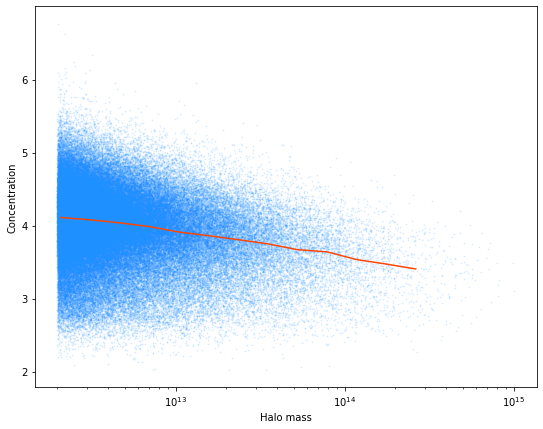
Let’s compute the mass-concentration relationship for halos in the halo light cone catalogs.
# compute mass and concentration proxy for all halos
halo_mass = cat.halos['N_interp'] * Mpart
concentration = cat.halos['r90_L2com'] / cat.halos['r25_L2com']

# select halos above 2.10^12 Msun/h (1000 particles)
mass_thresh = 2.0e12  # Msun/h
choice = halo_mass > mass_thresh

# compute median concentration
bins = np.logspace(11, 14.5, 21)
conc_median, _, inds = scist.binned_statistic(
    halo_mass[choice], concentration[choice], statistic='median', bins=bins
)
binc = (bins[1:] + bins[:-1]) * 0.5

# plot the mass vs. concentration relationship
plt.figure(figsize=(9, 7))
plt.scatter(
    halo_mass[choice], concentration[choice], s=1, alpha=0.1, color='dodgerblue'
)
plt.plot(binc, conc_median, color='orangered')
plt.xscale('log')
plt.xlabel('Halo mass')
plt.ylabel('Concentration')
Text(0, 0.5, 'Concentration')
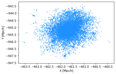
Let’s visualize the largest halo in this catalog.
# select the largest halo
i_max = np.argmax(halo_mass)
print(f'largest mass = {halo_mass[i_max]:.2e}')
start = cat.halos['npstartA'][i_max]
npout = cat.halos['npoutA'][i_max]
pos_max = cat.subsamples['pos'][start : start + npout]
plt.scatter(pos_max[:, 0], pos_max[:, 1], s=1, color='dodgerblue')
plt.xlabel('X [Mpc/h]')
plt.ylabel('Y [Mpc/h]')
largest mass = 1.00e+15
Text(0, 0.5, 'Y [Mpc/h]')
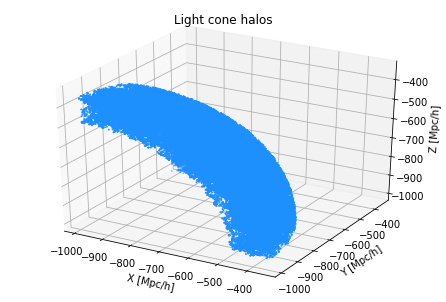
Finally, let’s plot the halos in this redshift catalog (they live in a thin shell that takes up an octant of the sky).
# plot the halos in this redshift catalog
halo_pos = cat.halos['pos_interp']

# creating figure
fig = plt.figure()
ax = Axes3D(fig)

# creating the plot
ax.scatter(
    halo_pos[choice, 0],
    halo_pos[choice, 1],
    halo_pos[choice, 2],
    s=1,
    color='dodgerblue',
)

# setting title and labels
ax.set_title('Light cone halos')
ax.set_xlabel('X [Mpc/h]')
ax.set_ylabel('Y [Mpc/h]')
ax.set_zlabel('Z [Mpc/h]')
Text(0.5, 0, 'Z [Mpc/h]')